Demonstration example of PVT interpolation

1 Overview
1.1 Example Target
This example is for the convenience of customer understanding, application of PVT interpolation function combined with the small stepper motor driver, the preliminary realization of the straight line drawing function through the mechanical arm. In the control part of this example, the embedded control module of a small stepper motor driver with high performance developed independently by Spectrum is used, and the precise control of the arm is realized by the motion control algorithm inside the module.
In order to understand the interpolation function of PVT, kinematics analysis of mechanical structure is needed in the early stage. This example gives a more detailed demonstration step for this mechanical structure, but due to the diversity of motion, in order to save space, only a detailed analysis of a certain motion situation is made.
Document description aims at PVT interpolation function of PSPMC007 series control module, including whole mechanism description, motion graph analysis, P position data analysis and V velocity data analysis.
2. Background description
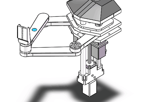
2.1 Equipment Mechanism Diagram

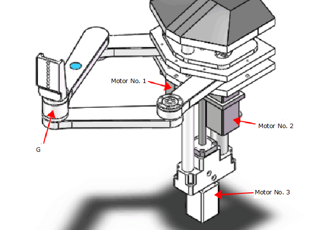
The mechanism is a three-axis manipulator arm, the 3rd motor controls the overall movement up and down, and the 1st and 2nd motors control the rotation of the two axes connected with them respectively, so that the accurate control of G-point can be realized. Then, in order to realize linear or circular motion of G-point, PVT interpolation is needed.

2.2 Introduction to PVT
PVT is an accurate interpolation method, which is widely used in trajectory planning of servo control system. PMC007 series small stepper motor driver receives a series of PVT points through CAN bus. Each PVT point is composed of position, speed and time. PMC007 controller interpolates these points precisely to get the required trajectory.
PVT synchronization control can not only ensure the smooth operation of the system, but also give full play to the potential of system resources, improve the average running speed of the system and system production efficiency, improve the control accuracy of the motion system as a whole, and make the acceleration curve transition smoothly at the inflection point. Reasonable interpolation control is an important link to ensure the dynamic performance and steady-state accuracy of high-speed motion system. PMC007 adopts PVT fine interpolation algorithm and makes use of the openness of the system to effectively combine the rough interpolation of the upper computer with the fine interpolation of the bottom controller. It not only makes the interpolation operation of the complex motion mechanism distributed in the industrial control network, but also greatly reduces the bus communication load, and makes the network synchronization control of the large number of nodes simple and reliable.
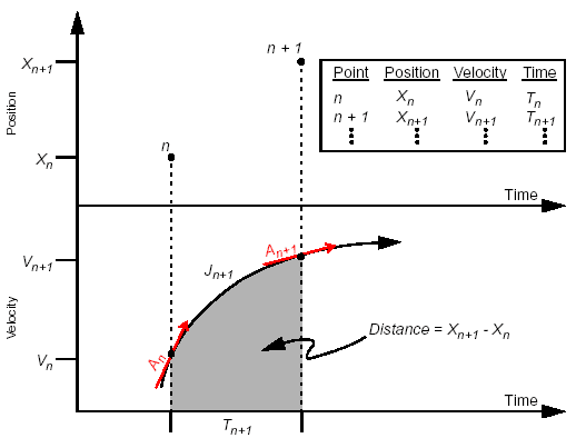
By setting a series of PVT points for the control module, the motors of each axis can pass or reach their respective target points at the same time (T), at their respective target velocities (V).
When in use, through the discretization of the continuous motion curve, continuous input PVT, can realize continuous motion of PVT, as shown below. The smaller the time interval of discretization (t) is (1ms (t 1s), the more the number of PVT points, the smoother the curve will be, but the greater the bandwidth pressure on the bus, so it is necessary to balance the load according to the number of axes on the network. The time interval T 20ms is usually used within three axes.

Graphical Analysis of Motion of 2.3 Mechanisms
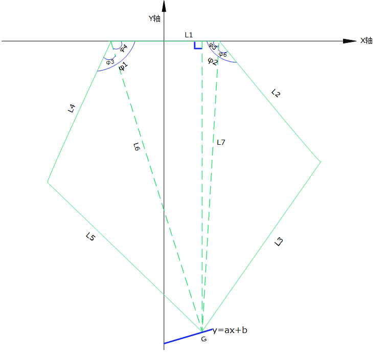
It can be seen from the graph that the difficulty in realizing the straight line or arc motion of G-point lies in the control of motor 1 and 2. Let motor 3 remain motionless for motion analysis. In this case, the overhead mechanism schematic diagram is shown as follows:

Linear interpolation:
To make G point go straight, the relation between coordinate X and Y is y = a x + B. Because of the particularity of the mechanism, the range of values of a, B and X is different, and the motion analysis is done only under the condition of 0.
When G-point goes straight, the correct PVT data of motor 1 and 2 need to be given by the system.
3.1 Location data (P) parsing:
1. Firstly, the line y = ax + B is divided into 5000 points in the range of 0. As long as G points pass through 5000 points in turn, the straight line trajectory can be formed. The corresponding x value is X0 X1 X2 X3... .X4999

2. To get the position data of No. 1 and No. 2 motors, it is necessary to get the angle of 1 and 2. The corresponding 1 and 2 values can be obtained by the x value of each point.
3.1.1 1 Value Solution
From the graph we can see that Phi 1 = Phi 3 + Phi 4
4 = arctan (-yL1+x)* (360/2pi) = arctan (-(ax+b) L1+x)* (360/2pi)
3 = arccos(L42+L62-L522*L4*L6)* (360/2pi)
= arccos(1+a2x2+2ab+2L1x+L42+L12+b2-L522*L4*1+a2x2+2ab+2L1x+L12+b2)* (360/2pi)
1= {arctan(-(ax+b)L1+x) +arccos(1+a2x2+2ab+2L1 x+L42+L12+b2-L522*L4*1+a2x2+2ab+2L1 x+L12+b2)}* (360/2pi)
3.1.2 2 Value Solution
5 = arctan (-yL1-x)* (360/2pi) = arctan (-(ax+b) L1-x)* (360/2pi)
6 = arccos(L22+L72-L322*L2*L7)* (360/2pi)
= arccos(1+a2x2+2ab-2L1x+L22+L12+b2-L322*L2*1+a2x2+2ab-2L1x+L12+b2)* (360/2pi)
2={arctan(-(ax+b)L1-x) +arccos1+a2x2+2ab-2L1 x+L22+L12+b2-L322*L2*1+a2x2+2ab-2L1 x+L12+b2}* (360/2pi)
3.21, 2 motor position algorithm
According to the value of x, the corresponding value of_1 and_2 can be calculated. Then, according to the angle difference between the value and the initial position value, the absolute positions of motor 1 and motor 2 can be obtained. Let the initial position angle of motor 1 be_10, and the initial position angle of motor 2 be_20.
The absolute position P of No. 1 motor is: 1-10/(1.8 subdivision)
The absolute position P of No. 2 motor is: 2-20/(1.8 subdivision)
3.3 Velocity Data (V) Analysis:
Angular derivation of time is angular velocity. Pulse frequency V can be obtained by angular velocity. Because there are many kinds of cases of drawing straight lines, here we only do analysis in the case of drawing straight lines at uniform speed. Let the velocity of drawing straight lines be V1.
Let P = 1 + a2x2 + 2Ab + 2L1x + L42 + L12 + B2 - L52
Q=2*L4*1+a2x2+2ab+2L1x+L12+b2
Angular Speed of Motor 3.3.11:
1 = d_1dt = (d_1dx)* (dxdt) = b-a*L1L1+x2+ax+b2-11-p2q2*21+a2x+2a b+2L1*q-2L42pq2*3602pi*V1*(-a b/b_+b_/a_)
3.3.12 Angular Speed of Motor:
Let u = 1+a2x2+2ab-2L1x+L22+L12+b2-L32
V = 2*L2*1+a2x2+2ab-2L1x+L12+b2
2 = D phi 2DT = (d phiphi 2D x) * (dxdt) = - b-a*L1L1-x 2+x+a x+a x+b2-11-u2v2*21+a2x+a2x+2a b-2b-2L1*v-2L22uvv2*3602pipipipi*V1*(-a b/b+b+b_+b_/a) QUOTarcE (- (a x+b) L1+a x+b) L1+b 1+l1+x) *+cos (1+arcaaaax+a x+2x+a2x+2x+a2x+42+L12+b2-L522*L4*1+a2x2+2a b+2L1 x+L12+b2)
Pulse Frequency (PPS) Algorithms for 3.41 and 2 Motors
The corresponding values of_1 and_2 are calculated according to the x value and the known V1 value, and the required PPS, i.e. the speed V, is converted according to the inherent properties of the motor.
Velocity V1 = _1* Subdivision of No.1 Motor
Velocity V2 = _2* Subdivision of No.2 Motor
4 Specific PVT data
See attached Excel form

Demonstration example of PVT interpolation

Login